# install.packages("AustralianPoliticians")
library(AustralianPoliticians)
library(lubridate)
library(tidyverse)
The average age of politicians in the Australian Federal Parliament (1901-2021)
I examine the average age of politicians in the Australian Federal Parliament on a daily basis. Using a publicly available dataset I find that generally the Senate is older than the House of Representatives. The average age increased from Federation in 1901 through to 1949, when an expansion of the parliament’s size likely brought many new politicians. I am unable to explain a sustained decline that occurred during the 1970s. From the 1980s onward there has been a gradual aging of both houses.
Overview
Last week I had the opportunity to attend my first thesis defence at a French-language institution (just to clarify - the actual defence was nonetheless conducted in English). Congratulations to Florence Vallée-Dubois on a successful defence. Her thesis looks at population ageing and democratic representation in Canada and is absolutely brilliant.
Her work, and some earlier comments by Ben Readshaw, got me thinking about what the average age of a politician in Australia looks like. Thankfully, this is an example of a question that my new R package with Paul Hodgetts AustralianPoliticians makes easy to answer (Alexander and Hodgetts 2021).
The average age of politicians in a parliament may have implications for the types of issues that are emphasised and the policies that are put in place. I examine the average age of Australian politicians in the Senate and the House of Representatives. In general, the Senate tends to be slightly older than the House of Representatives. I find a gradual increase in the average age from Federation through to the 1940s. In 1949 there was an expansion of the parliament and the average age noticeably declined. After a period of relative stability in the 1950s and 1960s, there was another noticeable decrease in the 1970s, followed by a gradual aging.
Data preparation
The dataset that I used in this note was primarily collected from records from the Australian Parliamentary Library, Wikipedia, and the Australian Dictionary of Biography. The dataset comprises biographical, political, and other information about every person elected to either the House of Representatives or the Senate. You can get the dataset in a series of CSVs on GitHub or as an R Package AustralianPoliticians available on CRAN.1
The other packages that are required for the analysis are lubridate (Grolemund and Wickham 2011), the tidyverse (Wickham et al. 2019). Additionally this note draws on the knitr (Xie 2020) and distill (Allaire et al. 2021) packages. All analysis is conducted in the statistical programming language R (R Core Team 2020).
I’m not going to spend a lot of time on descriptives about the dataset here because that’s needed for a paper, and this is meant to be fun.
all <- AustralianPoliticians::get_auspol("all")
head(all)
# A tibble: 6 × 20
uniqueID surname allOtherNames firstName commonName
<chr> <chr> <chr> <chr> <chr>
1 Abbott1859 Abbott Richard Hartley S… Richard <NA>
2 Abbott1869 Abbott Percy Phipps Percy <NA>
3 Abbott1877 Abbott Macartney Macartney Mac
4 Abbott1886 Abbott Charles Lydiard A… Charles Aubrey
5 Abbott1891 Abbott Joseph Palmer Joseph <NA>
6 Abbott1957 Abbott Anthony John Anthony Tony
# ℹ 15 more variables: displayName <chr>,
# earlierOrLaterNames <chr>, title <chr>, gender <chr>,
# birthDate <date>, birthYear <dbl>, birthPlace <chr>,
# deathDate <date>, member <dbl>, senator <dbl>,
# wasPrimeMinister <dbl>, wikidataID <chr>,
# wikipedia <chr>, adb <chr>, comments <chr>all$member %>% table().
0 1
578 1205 all$senator %>% table().
0 1
1155 628 But briefly, there are 1,783 politicians in the dataset, with 1,205 having sat in the House of Representatives, which is the lower house, and 628 having sat in the Senate, which is the upper house. There is some overlap because there are people who sat in both houses.2
The AustralianPoliticians package contains a number of datasets that are related by the uniqueID variable. This note requires the main dataset - ‘all’ - as well as two supporting datasets that provide more detailed information about the members - ‘mps’ - and the senators - ‘senators’.
# Get the members and the dates they were in the house
mps <- AustralianPoliticians::get_auspol("mps")

australian_mps <-
  all %>%
  filter(member == 1) %>%
  left_join(mps,
            by = "uniqueID") %>%
  select(uniqueID, mpFrom, mpTo) %>%
  mutate(house = "reps") %>%
  rename(from = mpFrom,
         to = mpTo)
# Get the senators and the dates they were in the senate
senators <- AustralianPoliticians::get_auspol("senators")
australian_senators <-
all %>%
filter(senator == 1) %>%
left_join(senators,
by = "uniqueID") %>%
select(uniqueID, senatorFrom, senatorTo) %>%
mutate(house = "senate") %>%
rename(from = senatorFrom,
to = senatorTo)
australian_politicians <- rbind(australian_mps, australian_senators)
rm(australian_senators, australian_mps, mps, senators)
# Change the names so that they print nicely in graphs/tables
australian_politicians <-
australian_politicians %>%
mutate(house =
case_when(
house == "senate" ~ "Senate",
house == "reps" ~ "HoR",
TRUE ~ "OH NO")
)
head(australian_politicians)# A tibble: 6 × 4
uniqueID from to house
<chr> <date> <date> <chr>
1 Abbott1869 1913-05-31 1919-11-03 HoR
2 Abbott1886 1925-11-14 1929-10-12 HoR
3 Abbott1886 1931-12-19 1937-03-28 HoR
4 Abbott1891 1940-09-21 1949-10-31 HoR
5 Abbott1957 1994-03-26 2019-05-18 HoR
6 Abel1939 1975-12-13 1977-11-10 HoR # australian_politicians$house %>% table()For each day, I would like to know the average age of everyone sitting in the parliament. There are a variety of ways to do this, but one is to create a dataset of two columns: date and uniqueID. Both of these are repeated, so that for every date there is every uniqueID.
start_date <- ymd("1901-01-01")
end_date <- ymd("2021-12-31")

politicians_by_date <-
  tibble(
    uniqueID = rep(australian_politicians$uniqueID %>% unique(),
                   end_date - start_date + 1),
    date = rep(seq.Date(start_date, end_date, by = "day"),
               australian_politicians$uniqueID %>% unique() %>% length()
               )
    )

head(politicians_by_date)
# A tibble: 6 × 2
uniqueID date
<chr> <date>
1 Abbott1869 1901-01-01
2 Abbott1886 1901-01-02
3 Abbott1891 1901-01-03
4 Abbott1957 1901-01-04
5 Abel1939 1901-01-05
6 Adams1951 1901-01-06Although the dataset is long at this point, it will be quite sparse as there are many combinations of date and uniqueID that are irrelevant. In the next step I check if each uniqueID was in parliament on each date, and filter away those that were not.
# Add an explicit end date to the uniqueIDs that are still in parliament and
# hence have NA in the date they left parliament.
australian_politicians$to[is.na(australian_politicians$to)] <- end_date

politicians_by_date <-
  politicians_by_date %>%
  left_join(australian_politicians,
            by = "uniqueID"
            )
Warning in left_join(., australian_politicians, by = "uniqueID"): Detected an unexpected many-to-many relationship between
`x` and `y`.
ℹ Row 1 of `x` matches multiple rows in `y`.
ℹ Row 1 of `y` matches multiple rows in `x`.
ℹ If a many-to-many relationship is expected, set
`relationship = "many-to-many"` to silence this warning.politicians_by_date <-
politicians_by_date %>%
mutate(in_parliament_interval = interval(from, to),
in_parliament_at_date = if_else(date %within% in_parliament_interval,
1,
0)
) %>%
filter(in_parliament_at_date == 1) %>%
select(-in_parliament_interval,
-in_parliament_at_date,
-from,
-to)
head(politicians_by_date)# A tibble: 6 × 3
uniqueID date house
<chr> <date> <chr>
1 Bonython1848 1901-04-13 HoR
2 Braddon1829 1901-04-25 HoR
3 Brown1861 1901-05-11 HoR
4 Cameron1851 1901-06-13 HoR
5 Chanter1845 1901-07-13 HoR
6 Chapman1864 1901-07-14 HoR Now that the dataset is a bit more tractable, I add the birthday of every uniqueID and then calculate their age, in days, for every date.
politicians_by_house_and_birthday <-
  all %>%
  select(uniqueID, birthDate, member, senator) %>%
  pivot_longer(cols = c(member, senator),
               names_to = "house",
               values_to = "in_it"
               ) %>%
  filter(in_it == 1) %>%
  select(-in_it) %>%
  mutate(house =
           case_when(
             house == "senator" ~ "Senate",
             house == "member" ~ "HoR",
             TRUE ~ "OH NO")
         )

# Check if the catch-all has been invoked
# politicians_by_house_and_birthday[politicians_by_house_and_birthday$house == "OH NO",]

politicians_by_date <-
  politicians_by_date %>%
  left_join(politicians_by_house_and_birthday,
            by = c("uniqueID", "house")
            )

politicians_by_date <-
  politicians_by_date %>%
  filter(!is.na(birthDate)) %>% # I can't find Trish Wortley's birthday and also
  # we don't know the birthdates of some of the politicians from around Federation.
  mutate(age_as_at_that_date = date - birthDate)

head(politicians_by_date)
# A tibble: 6 × 5
uniqueID date house birthDate age_as_at_that_date
<chr> <date> <chr> <date> <drtn>
1 Bonython1… 1901-04-13 HoR 1848-10-15 19172 days
2 Braddon18… 1901-04-25 HoR 1829-06-11 26250 days
3 Brown1861 1901-05-11 HoR 1861-10-06 14461 days
4 Cameron18… 1901-06-13 HoR 1851-11-03 18119 days
5 Chanter18… 1901-07-13 HoR 1845-02-11 20605 days
6 Chapman18… 1901-07-14 HoR 1864-07-10 13517 days I need to work out the average age for each day. There are some politicians for whom we do not know their exact birthdate. Those have been removed in this calculation.
average_age_by_date <-
  politicians_by_date %>%
  mutate(age_as_at_that_date = age_as_at_that_date / ddays(1)) %>% # This just converts it into a days count
  group_by(date, house) %>%
  summarise(average_age = median(age_as_at_that_date, na.rm = TRUE))
`summarise()` has grouped output by 'date'. You can
override using the `.groups` argument.average_age_by_date <-
average_age_by_date %>%
mutate(average_age_in_years = average_age/365)
head(average_age_by_date)# A tibble: 6 × 4
# Groups: date [3]
date house average_age average_age_in_years
<date> <chr> <dbl> <dbl>
1 1901-03-29 HoR 16765 45.9
2 1901-03-29 Senate 16086. 44.1
3 1901-03-30 HoR 17235 47.2
4 1901-03-30 Senate 18878. 51.7
5 1901-03-31 HoR 17236 47.2
6 1901-03-31 Senate 18878. 51.7I’ll do the same thing except to work out the average by election period. This requires grabbing the election periods (there’s an R package coming soon about this)!
elections <- read_csv("https://raw.githubusercontent.com/RohanAlexander/australian_federal_elections/master/outputs/elections.csv",
                      col_types = "Dicc")

average_age_by_election <-
  politicians_by_date %>%
  left_join(elections %>%
              rename(date = electionDate) %>%
              select(-comment) %>%
              mutate(house = "HoR"),
            by = c("date", "house")) %>%
  ungroup() %>%
  filter(house == "HoR") %>%
  arrange(date, uniqueID) %>%
  mutate(is_election = if_else(is.na(electionWinner), 0, 1),
         is_election = if_else(is_election == lag(is_election, default = 0), 0, is_election),
         election_counter = cumsum(is_election))

average_age_by_election <-
  average_age_by_election %>%
  ungroup() %>%
  mutate(age_as_at_that_date = age_as_at_that_date / ddays(1)) %>% # This just
  # converts it into a days count
  group_by(election_counter) %>%
  summarise(average_age = median(age_as_at_that_date, na.rm = TRUE),
            first_date = min(date)) %>%
  mutate(average_age_in_years = average_age/365) %>%
  ungroup()
Results
Over time
There are considerable changes over time (Figure @ref(fig:maingraph)).
average_age_by_date %>%
  # filter(year(date) == 1904) %>%
  # filter(month(date) == 2) %>%
  # filter(house == "HoR") %>%
  ggplot(aes(x = date, y = average_age_in_years, colour = house)) +
  geom_point(alpha = 0.5) +
  labs(x = "Date",
       y = "Average age (years)",
       color = "House") +
  theme_minimal() +
scale_color_brewer(palette = "Set1") 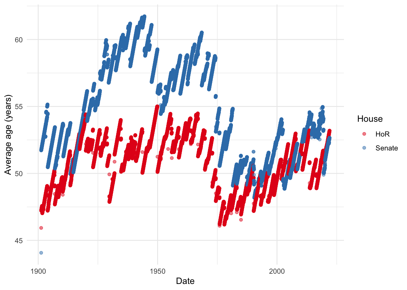
I’ll just separate each of the houses because there’s a lot going on there (Figures @ref(fig:justrepsthings) and @ref(fig:justsenatethigns)).
average_age_by_date %>%
  filter(house == "HoR") %>%
  ggplot(aes(x = date, y = average_age_in_years)) +
  geom_point(alpha = 0.5, color = "#F90000") +
  labs(x = "Date",
       y = "Average age (years)") +
  theme_minimal() +
scale_color_brewer(palette = "Set1") 
average_age_by_date %>%
  filter(house == "Senate") %>%
  ggplot(aes(x = date, y = average_age_in_years)) +
  geom_point(alpha = 0.5, color = "#0080BD") +
  labs(x = "Date",
       y = "Average age (years)") +
  theme_minimal() +
scale_color_brewer(palette = "Set1") 
Group by election period
We can also look at a summary of the results, averaged across days, on the basis of each election period (Table @ref(tab:maintable) and Figure @ref(fig:othergraph)).
average_age_by_election %>%
  select(-average_age) %>%
  rename(`Election number` = election_counter,
         `Period begins` = first_date,
         `Average age (years)` = average_age_in_years) %>%
  kable(caption = "Average age by for each period between lower house elections",
        digits = 1,
booktabs = TRUE)| Election number | Period begins | Average age (years) |
|---|---|---|
| 1 | 1901-03-29 | 48.2 |
| 2 | 1903-12-16 | 48.8 |
| 3 | 1906-12-12 | 49.0 |
| 4 | 1910-04-13 | 50.1 |
| 5 | 1913-05-31 | 49.8 |
| 6 | 1914-09-05 | 51.9 |
| 7 | 1917-05-05 | 53.0 |
| 8 | 1919-12-13 | 52.2 |
| 9 | 1922-12-16 | 51.7 |
| 10 | 1925-11-14 | 52.3 |
| 11 | 1928-11-17 | 50.9 |
| 12 | 1929-10-12 | 49.4 |
| 13 | 1931-12-19 | 52.3 |
| 14 | 1934-09-15 | 51.1 |
| 15 | 1937-10-23 | 51.9 |
| 16 | 1940-09-21 | 52.2 |
| 17 | 1943-08-21 | 51.6 |
| 18 | 1946-09-28 | 53.3 |
| 19 | 1949-12-10 | 50.9 |
| 20 | 1951-04-28 | 52.4 |
| 21 | 1954-05-29 | 53.7 |
| 22 | 1955-12-10 | 52.4 |
| 23 | 1958-11-22 | 52.5 |
| 24 | 1961-12-09 | 53.5 |
| 25 | 1963-11-30 | 53.5 |
| 26 | 1966-11-26 | 52.5 |
| 27 | 1969-10-25 | 51.3 |
| 28 | 1972-12-02 | 49.5 |
| 29 | 1974-05-18 | 48.6 |
| 30 | 1975-12-13 | 47.1 |
| 31 | 1977-12-10 | 47.3 |
| 32 | 1980-10-18 | 48.3 |
| 33 | 1983-03-05 | 47.7 |
| 34 | 1984-12-01 | 48.2 |
| 35 | 1987-07-11 | 49.4 |
| 36 | 1990-03-24 | 48.5 |
| 37 | 1993-03-13 | 48.9 |
| 38 | 1996-03-02 | 48.9 |
| 39 | 1998-10-03 | 49.7 |
| 40 | 2001-11-10 | 50.7 |
| 41 | 2004-10-09 | 51.7 |
| 42 | 2007-11-24 | 51.2 |
| 43 | 2010-08-21 | 51.5 |
| 44 | 2013-09-07 | 50.0 |
| 45 | 2016-07-02 | 50.2 |
| 46 | 2019-05-18 | 51.7 |
average_age_by_election %>%
  ggplot(aes(x = first_date, y = average_age_in_years)) +
  geom_point() +
  labs(x = "Date",
       y = "Average age (years)") +
  theme_minimal() +
scale_color_brewer(palette = "Set1") 
Compare with average age
To get a sense of whether the parliament is unusual we need know what is happening the broader population over this time. Fortunately, I know someone who is fairly handy when it comes to demography who can help.3
Although it’s going to average over elections, which we’ve seen is a big source of variation, we can create an average age for each year, and then compare that against data from the Australian Bureau of Statistics (ABS). The ABS provides an estimate of historical population statistics in 3105.0.65.001 - Australian Historical Population Statistics, 2016, which was released in 2019. I want the second data cube - 2 - Population Age and Sex Structure - and within that I want Table 2.18 - Median age by sex, states and territories, 30 June, 1861 onwards.
library(readxl)
library(janitor)
Attaching package: 'janitor'The following objects are masked from 'package:stats':
chisq.test, fisher.testABS_data <- read_excel("3105065001ds0002_2019.xls",
sheet = "Table 2.18",
skip = 4) %>%
janitor::clean_names() %>%
rename(area_and_type = x1,) %>%
select(-x1861, -x1870, -x1871, -x1881, -x1891)New names:
• `` -> `...1`ABS_data <-
ABS_data %>%
mutate(type = ifelse(area_and_type %in% c("Males", "Females", "Persons"), area_and_type, NA),
area_and_type = ifelse(is.na(type), area_and_type, NA)) %>%
select(area_and_type, type, everything()) %>%
fill(area_and_type, .direction = "down") %>%
mutate(area_and_type = str_remove(area_and_type, "\\(f\\)\\(g\\)"))
ABS_data <-
ABS_data %>%
filter(area_and_type == "Australia",
type == "Persons")
ABS_data <-
ABS_data %>%
pivot_longer(cols = starts_with("x"),
names_to = "year",
values_to = "median") %>%
mutate(year = str_remove(year, "x"),
year = as.integer(year)) %>%
rename(area = area_and_type)average_age_by_year <-
politicians_by_date %>%
ungroup() %>%
mutate(year = year(date)) %>%
mutate(age_as_at_that_date = age_as_at_that_date / ddays(1)) %>% # This just
# converts it into a days count
group_by(year) %>%
summarise(average_age = median(age_as_at_that_date, na.rm = TRUE)) %>%
mutate(average_age_in_years = average_age/365) %>%
ungroup() average_age_by_year %>%
left_join(ABS_data, by = "year") %>%
select(year, average_age_in_years, median) %>%
rename(Politicians = average_age_in_years,
Overall = median) %>%
pivot_longer(cols = c(Politicians, Overall),
names_to = "population",
values_to = "median") %>%
ggplot(aes(x = year, y = median, color = population)) +
geom_point() +
# geom_smooth() +
theme_classic() +
scale_color_brewer(palette = "Set1") +
labs(x = "Year",
y = "Median age (years)",
color = "Population")Warning: Removed 23 rows containing missing values
(`geom_point()`).
Concluding remarks
I’ve had a brief look at the average age of politicians in the Australian Parliament. In general, I’ve found that they’re older than the general population, and that there’s a lot of variation.
More generally, I’ve shown one of the advantages of putting data onto GitHub, and wrapping that in an R Package where possible. If you don’t like my analysis then you can grab the data yourself and play around with it!
As I mentioned at the top, Florence Vallée-Dubois does a lot more of this type of work in her thesis ‘Growing old : Population ageing and democratic representation in Canada’ where she looks at ‘whether the social changes brought about by population ageing also have implications for electoral politics and democratic representation.’ There’s probably a lot of similar work that could be done for Australia.
Acknowledgments
Thanks very much to Ben Readshaw and Florence Vallée-Dubois for motivating this note, and to Monica Alexander for her thoughtful comments.
References
Alexander, Rohan, and Paul A. Hodgetts. 2021. AustralianPoliticians: Provides Datasets about Australian Politicians. https://CRAN.R-project.org/package=AustralianPoliticians.
Allaire, JJ, Rich Iannone, Alison Presmanes Hill, and Yihui Xie. 2021. Distill: ’R Markdown’ Format for Scientific and Technical Writing. https://CRAN.R-project.org/package=distill.
Grolemund, Garrett, and Hadley Wickham. 2011. “Dates and Times Made Easy with lubridate.” Journal of Statistical Software 40 (3): 1–25. https://www.jstatsoft.org/v40/i03/.
R Core Team. 2020. R: A Language and Environment for Statistical Computing. Vienna, Austria: R Foundation for Statistical Computing. https://www.R-project.org/.
Wickham, Hadley, Mara Averick, Jennifer Bryan, Winston Chang, Lucy D’Agostino McGowan, Romain François, Garrett Grolemund, et al. 2019. “Welcome to the tidyverse.” Journal of Open Source Software 4 (43): 1686. https://doi.org/10.21105/joss.01686.
Xie, Yihui. 2020. Knitr: A General-Purpose Package for Dynamic Report Generation in r. https://yihui.org/knitr/.
Footnotes
Monica Alexander uses an early version of this dataset to look at the average age of death of Australian politicians: https://www.monicaalexander.com/posts/2019-08-09-australian_politicians/.↩︎
There are a handful of politicians who sat in the parliament, but were never elected - when the first parliament sat, there were initially some who were just appointed, and never went on to seek election. Conversely, there is one politician - Heather Hill - who was elected, but whose election was reversed before she could take her seat. While she never served in either house, she is included in the dataset for purposes of being able to link it to the elections dataset. However she is not included in the number of Australian politicians.↩︎
If you’re interested in this sort of thing, then a PhD with Monica Alexander is probably the way to go.↩︎